Task: To simultaneously deblur and supersample prostate specific membrane antigen (PSMA) positron emission tomography (PET) images using neural blind deconvolution
Description: Blind deconvolution is a method of estimating the hypothetical ‘deblurred’ image along with the blur kernel (related to the point spread function) simultaneously. Traditional maximum a posteriori blind deconvolution methods require stringent assumptions and suffer from convergence to a trivial solution. A method of modelling the deblurred image and kernel with independent neural networks, called ‘neural blind deconvolution’ had demonstrated success for deblurring 2D natural images in 2020. The Neural_Blind_DeConv_PSMA model adapts neural blind deconvolution to specifically deblur PSMA PET images while attaining simultaneous supersampling to double the original resolution.
Neural blind deconvolution, as first demonstrated by Ren et al (Ext. Ref.), estimates a deblurred version, x, of an actual image, y, by training neural networks on a case-specific basis. Specifically, two neural networks, Gx and Gk are trained to predict x, and a blur kernel, k, whose convolution together yields a close estimate of the original image, y.
Neural blind deconvolution was originally demonstrated on 2D images using a ‘U-Net’ (Ronneberger et al Ext. Ref.)-style, symmetric, multiscale, autoencoder network for Gx and a shallow fully-connected network for Gk . The developers of Neural_Blind_DeConv_PSMA model built off of this methodology while implementing some notable changes to optimize model performance on PSMA PET images. A schematic diagram of the network design is shown below:
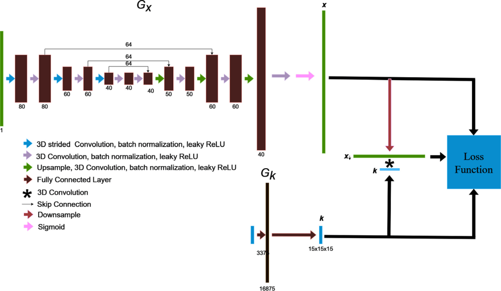
The blind deconvolution architecture used for deblurring PSMA PET images is illustrated. Gx is an asymmetric, convolutional auto-encoder network for predicting the deblurred image, x , and Gk is a fully-connected network for predicting the blur kernel, k . The convolution of x and k is trained to match the original image by using back-propagated model gradients from the loss function for iterative optimization
Unlike conventional supervised learning algorithms, separating training from validation datasets is not necessary for this type of models. Neural blind deconvolution is a type of ‘zero shot’ (Shocher et al Ext. Ref.) self-supervised learning algorithm, which utilises deep learning without requiring prior model training. Instead, parameters of Gx and Gk are optimized separately for each individual patient to predict the deblurred images. The algorithm for updating network weights to predict deblurred PSMA PET images is summarized below:
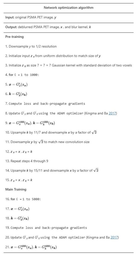
The optimization algorithm for updating network weights to predict deblurred PSMA PET images. It builds off of Ren et al’s proposed joint optimization algorithm (Ext. Ref.) implementing modifications by Kotera et al (Ext. Ref.).
Evaluation: The methodology is compared against several interpolation methods in terms of resultant blind image quality metrics. The Neural_Blind_DeConv_PSMA model’s ability is tested to predict accurate kernels by re-running the model after applying artificial ‘pseudokernels’ to deblurred images. The methodology was tested on a retrospective set of 30 prostate patients as well as phantom images containing spherical lesions of various volumes.
Results: The Neural_Blind_DeConv_PSMA model led to improvements in image quality over other interpolation methods in terms of blind image quality metrics, recovery coefficients, and visual assessment. Deblurred images had higher BRISQUE and CLIP scores than original images upsampled using nearest-neighbours, linear, quadratic, and cubic interpolation.
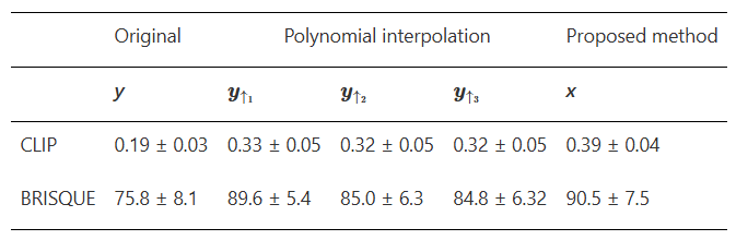
Blind image quality metrics, CLIP and BRISQUE are compared for original (y) and deblurred (x) PSMA PET images. For appropriate comparison, y was upsampled by 2 in each dimension to match the size of x. In the first column, y is upsampled using nearest neighbours interpolation to remain visually identical. The quality of y is also compared when upsampled using linear, quadratic and cubic interpolation
Maximum intensity projections of x , k , x * k , and y are shown for a single patient in figure below
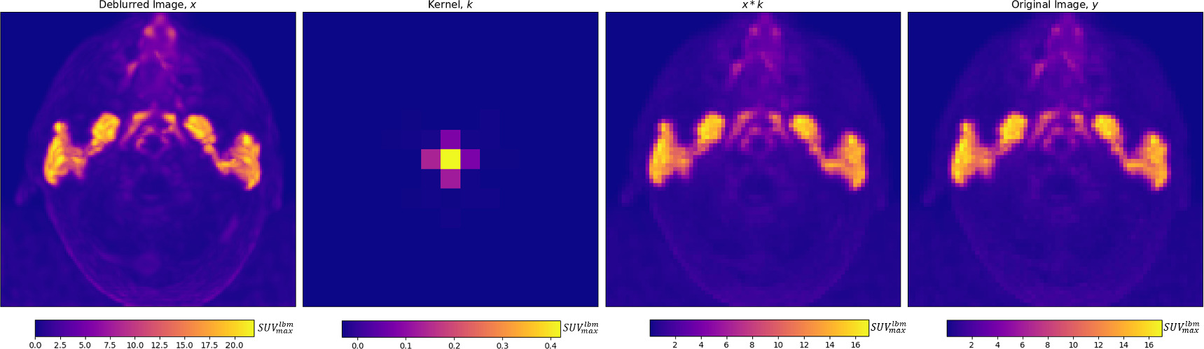
From left to right, for an individual patient, a deblurred maximum intensity projection image, and axial projection of the predicted kernel are shown, along with the maximum intensity projection of the convolution of the deblurred image and kernel, which is trained to match the original image, on the right
Visual comparisons of original and deblurred PET image slices including parotid glands and submandibular glands are shown for 3 different patients in figure below

Axial slices intersecting parotid glands (left) and submandibular glands (right) for 3 different patients are shown on original and deblurred images
Maximum intensity projection images are shown through the head and neck in figure below.
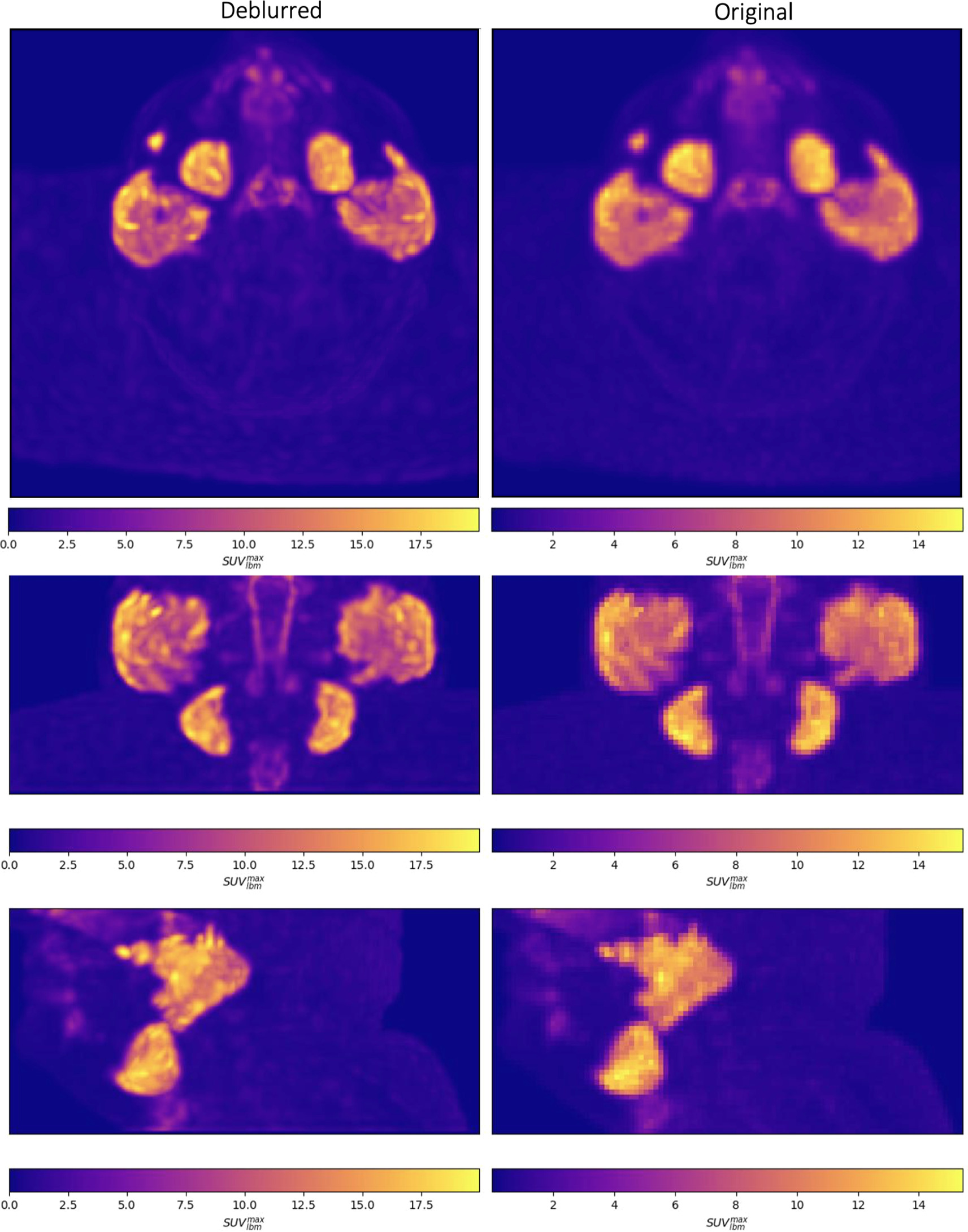
Maximum intensity projections of deblurred (left) and original (right) PSMA PET images are shown through the head and neck in the axial (top), coronal (middle) and sagittal (bottom) planes
Predicted kernels were similar between patients, and the model accurately predicted several artificially-applied pseudokernels.
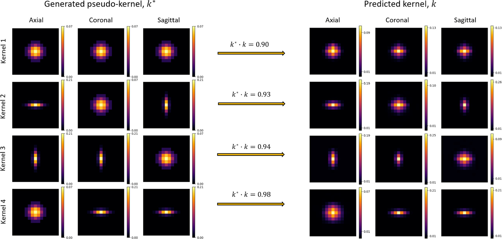
To validate the model’s ability to predict accurate blur kernels, 4 variously skewed pseudokernels were applied to deblurred images before re-running the blind deconvolution. Generated pseudokernels (k*, left) and their corresponding predicted kernel (k, right) are shown in separate rows for each of the 4 pseudokernel shapes, in axial, coronal, and sagittal image slices. The dot-product of normalized kernels, k* · k, was used to assess kernel similarity
Localization of activity in phantom spheres was improved after deblurring, allowing small lesions to be more accurately defined. Axial MIPs and slices of original and deblurred phantom images are shown in figure below. Activity concentrations were more localized within spheres after deblurring. This was most pronounced in small spheres (≤10 mm).
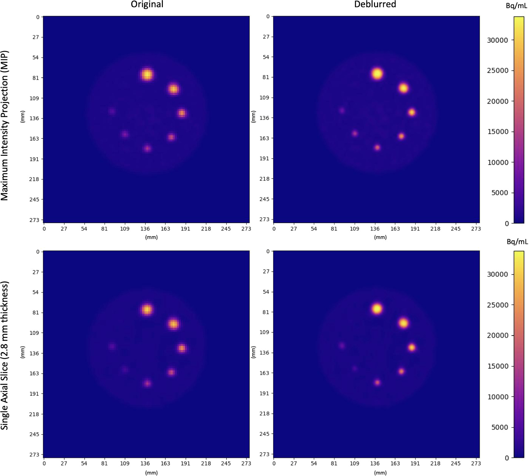
Original and Deblurred PET images of the Q3P phantom. Coplanar spheres containing uniform 22NaCl activity concentrations fused in epoxy resin are seen in a single axial slice. Clockwise from the top sphere, diameters were 16 mm, 14 mm, 10 mm, 8 mm, 7 mm, 6 mm, 5 mm. Spheres appear more homogeneous and localized (especially in smaller regions) after deblurring
Claim: The intrinsically low spatial resolution of PSMA PET leads to partial volume effects (PVEs) which negatively impact uptake quantification in small regions. The proposed Neural_Blind_DeConv_PSMA model can be used to mitigate this issue, and can be straightforwardly adapted for other imaging modalities. The developers have adapted neural blind deconvolution for simultaneous PVE correction and supersampling of 3D PSMA PET images. PVE correction allows for fine detail recovery within the imaging field, such as uptake patterns within salivary glands. Leveraging the power of deep learning without the need for a large training data set or prior probabilistic assumptions makes neural blind deconvolution a powerful PVE correction method. Their results demonstrate improvements in the method’s ability to improve image quality over other commonly used supersampling techniques
Dataset: Full-body [18F]DCFPyL PSMA PET/CT images were de-identified for 30 previous prostate cancer patients (mean age 68, age range 45–81; mean weight: 90 kg, weight range 52–128kg). Patients had been scanned, two hours following intravenous injection, from the thighs to the top of the skull on a GE Discovery MI (DMI) scanner. The mean and standard deviation of the injected dose was 310 ± 66 MBq (minimum: 182 MBq, maximum: 442 MBq). PET images were reconstructed using VPFXS (OSEM with time-of-flight and point spread function corrections) (number of iterations/subsets unknown, pixel spacing: 2.73/3.16 mm, slice thickness: 2.8/3.02mm). The scan duration was 180 s per bed position. For appropriate comparison of voxel values between patients, patient images were all resampled to a slice thickness of 2.8 and pixel spacing of 2.73 using linear interpolation. Helical CT scans were acquired on the same scanner (kVP: 120, pixel spacing: 0.98 mm, slice thickness: 3.75 mm).
Images were cropped to within 6 slices below the bottom of the submandibular glands and 6 slices above the top of the parotid glands. Cropping was employed to avoid exceeding time constraints and the 6 GB memory of the NVIDIA GeForce GTX 1060 GPU used for training. Registered CT images were used to contour parotid and submandibular glands for calculating uptake statistics. Limbus AI (Wong et al Ext. Ref.) was used for preliminary auto-segmentation of the glands on CT images, which were then manually refined by a single senior Radiation Oncologist, Jonn Wu. Contours were used to calculate uptake statistics within salivary glands. Images were normalized to the maximum voxel value prior to deblurring, and afterwards rescaled to standard uptake values normalized by lean body mass (SUVlbm). Lean body mass was estimated from patient weight and height using the Hume formula (Hume Ext. Ref.).
Remarks: The ill-posed problem of simultaneously estimating the theoretical ‘deblurred’ image, x , along with the spread-function or blur kernel, k , from the original image y ( y = x∗k ), is referred to as blind deconvolution. Traditional maximum a posteriori (MAP)-based methods for solving blind deconvolution require estimation of prior distributions for the kernel and deblurred image and specialized optimization techniques to avoid convergence towards a trivial solution. MAP-based methods are governed by the equation

where Pr(y∣k∣x) is the fidelity term likelihood and Pr(x) and Pr(k) are the priors of the deblurred image and blur kernel, respectively. In 2020, Ren et al (Ext. Ref.) developed ‘neural blind deconvolution’ for estimating the deblurred image and blur kernel from 2D natural images using two neural networks which are optimized simultaneously, as opposed to traditional MAP-based methods which generally employ alternating optimization to avoid a trivial solution (Ren et al Ext. Ref.). This is a self-supervised deep learning method that does not involve a separate training set, but instead learns to predict deblurred images independently for each image. Neural blind deconvolution was shown to out-perform (Ren et al Ext. Ref.) other traditional methods in terms of peak signal-to-noise ratio, SSIM, and error ratio.
The Neural_Blind_DeConv_PSMA model is built off of the development of 2D neural blind deconvolution (Ren et al Ext. Ref., Kotera et al Ext. Ref.), implementing changes to the network architecture and optimization procedures for suitability with 3D PSMA PET medical images. The developers also modify the architecture to accomodate simultaneous supersampling to enhance spatial resolution.
Original Neural Blind Deconvolution Neural Network Publication
